Subsections of System Design
Demand Side Platform
Subsections of Demand Side Platform
Artisan vs Optimizable Targetings
Demand-Side Platforms (DSP) and AdExchange targetings can get really complex really fast, especially when your DSP or AdExchange starts implementing machine learning features like CTR optimization and CPC bidding strategies. But when you’re just starting, it’s very easy.
The Artisan Approach to Targeting
You add geo-targeting. Some domain targetings. Some app targetings. Device type (phone/tablet/CTV), OS, browser, OS version. Device brand and make.
But then it gets a bit more evolved. Custom targeting for battery level, connection type—what have you.
Also, creatives need targetings too. VPAID video creatives will need protocol support and supported media types checked, bitrates validated, length of the video. Even more involved for display creatives: Do we need MRAID support? Do we match on exact dimensions or will bigger ones work just as well for us?
The same thing applies to DSP-wide filtering of traffic—all those dozens of blocklists: domains, apps, CIDRs and individual IPs, user agents of crawlers, and publisher IDs.
And if you’re starting from scratch or inherited a well-established bidder, it’s very likely that each targeting is carefully coded from scratch—all the way from UI frontend, UI backend, config update, ingestion, and implementation in the bidder.
I call it an artisan approach—carefully handcrafted parts intricately woven together to deliver a luxury experience. This is one way to go. It works.
Targetings And Time
But with time, what tends to happen is that the number of campaigns grows fast. At first, it’s hundreds, and after just a few short years, it’s already thousands. The number of targetings grows. They start to take more time in the flame graph or CPU time top in pprof. And you notice that the structure of targetings is quite stable, but with time and new SSPs, targetings start to contain an enormous amount of business logic about variations between SSPs.
Usually, they are evaluated one campaign at a time, going through all of the targetings, all the way down. And the main optimization is to put on top of the funnel the “cheap” ones or the ones that would filter out most of the campaigns (think device type, or is it video, or is it in-app/web, mobile/desktop, etc.).
Patterns in Targetings
So what is an alternative?
Well, it’s easy to start noticing that targetings have a very regular structure that really stems from the fact that we match a value at different paths in an OpenRTB object to the campaign requirements.
Most targetings are about checking inclusion of a particular field in a set. Think domain allowlist of a campaign or a set of device types (phones, tablets) that the campaign is targeting.
Sometimes it’s a “negative targeting,” which is about checking if a field does not match.
And most fields are ints, strings, or lists of strings and ints. Rarely are these boolean types or floats.
I’m pretty sure you can see where I’m going with this.
Optimizable Approach to Targeting
Yes. Autogenerate all the targetings. They are going to be simple. But it’s possible to get them for literally every field.
There are nuances, as usual. Geo is usually about a hierarchy. There’s London, Ontario, and London, UK. These are two very different Londons. There’s Vancouver, BC, and Vancouver, WA. These things are important.
And if your DSP implements geofencing/supergeo targeting that is based on user coordinates, that’ll be inevitably complex.
So while the autogenerated targetings work fine, you will have to accommodate custom ones. Which would be wise, given that pacing, budget capping, and predictive targetings will have to be a part of a campaign’s filtering funnel.
Simplifying the Filtering Funnel
Usually, the filtering funnel is very simple, just a logical AND between conditions:
targeting1 AND targeting2 AND targeting3...
That’s simple enough. Sometimes you can throw in an OR.
And strictly speaking, if you go for autogenerated targetings with well-defined interfaces, implementing arbitrary logical expressions becomes possible.
In practice, a simple chain of targetings with “AND” works just fine. And also, arbitrary formulas are hard to represent in the UI—or rather, hard to have a good UX with these formulas.
Exploring Logical Expressions in Targetings
On the other hand, that opens interesting possibilities:
For the geo matching above, we can actually represent targeting as:
(device.city == 'London' AND device.region == "Ontario" AND device.country == "Canada") OR (...)
And of course, the representation of targetings doesn’t need to look like that—at all.
{
  "targeting": {
    "Or": {
      "conditions": [
        {
          "And": {
            "conditions": [
              {
                "StringListMatch": {
                  "path": ".device.geo.city",
                  "match": [
                    "London"
                  ]
                }
              },
              {
                "StringListMatch": {
                  "path": ".device.geo.region",
                  "match": [
                    "Ontario"
                  ]
                }
              },
              {
                "StringListMatch": {
                  "path": ".device.geo.country",
                  "match": [
                    "Canada"
                  ]
                }
              }
            ]
          }
        }
      ]
    }
  }
}
But this particular approach with the arbitrary targeting formulas can be unnecessarily complicated and lead to optimizing trees of logical expressions. I think it might be optimized in simpler ways if we stick to a classical targeting filtering funnel with a single AND between a long list of matching predicates.
{
  "targeting": {
    "And": {
      "conditions": [
        {
          "IntListMatch": {
            "path": ".device.devicetype",
            "match": [
              1,
              4,
			  5
            ]
          }
        },
        {
          "IntListMatch": {
            "path": ".at",
            "match": [
              2
            ]
          }
        },
        {
          "StringListMatch": {
            "path": ".device.os",
            "match": [
              "iOS"
            ]
          }
        }
      ]
    }
  }
}
Sorry for the verbose listing, but you can see that this can be very easily deserialized from JSON and evaluated as fast as “artisan” targetings (well, if we don’t go fancy into arbitrary logical formulas).
Optimizing Targetings
I call this approach “optimizable” rather than autogenerated because this kind of regular structure lends itself naturally to optimization.
As an example, in a logical AND at runtime, we can, with some sampling, measure how long each of the condition evaluations takes and how frequently they reject the request.
And we can order conditions in the logical AND expression by the expected rejection cost: P(reject) * CPU time, to get the cheapest rejects to the top of a filtering funnel.
Individual targetings can be optimized as well in an automated manner, especially those with low cardinality. And geo might deserve special treatment, after all.
And this is what I want to talk about next time.
Optimizing Targetings
One of the oldest ideas for the optimization of targetings is to use reverse indices.
I worked in a few companies over 15 years ago, and they utilized it to their benefit. But the first time I read about it, though, was in an O’Reilly book on the use of Redis, just a few years ago. You can look it up there.
However, here it is with a very simple approach.
Campaign Example
Imagine that you have an ad network that has only demographic information about the users, and campaigns use age and gender targeting.
(And this is a formulation I had when I interviewed for my first adtech job, where I was able to come up with a concept by the end of a 4-hour interview. And I’m still grateful to this company and the amazing people I met there.)
So let’s talk about the campaigns for a while.
- Campaign 1 targets male audience between ages 35 and 40.
- Campaign 2 targets people between 21 and 40.
- Campaign 3 has no targetings (it’s a catch-all campaign).
And there are 10k campaigns like that.
So what would be an efficient way to match campaigns, so that we can choose between them?
Creating Reverse Indices with Bitsets
The answer is simple. We create reverse indices!
For age:
- 21 → bitset of campaigns targeting 21-year-olds
- 22 → bitset of campaigns targeting 22-year-olds
- …
- 40 → bitset of campaigns targeting 40-year-olds
- And, a bitset of campaigns that have no age targeting
For gender:
- male → bitset of campaigns targeting male audience
- female → bitset of campaigns targeting female audience
- other → bitset of campaigns targeting ‘other’ audience
- And, a bitset of campaigns that have no gender targeting
When we create bitsets, for simplicity, we can just assume that we have 10k campaigns, and they are numbered from 0 to 9999. And when campaigns 1 and 2 target 36-year-olds, the bits 1 and 2 will be set in a 10k-bit-long bitset.
Applying Targetings
So let’s say we have a 22-year-old male. To find all the campaigns that match, we just need to do two things:
-
Find these bitsets:
- Bitset for 22-year-olds (
bitset(age, 22)) - Bitset for campaigns without age targeting (
bitset(age, any)) - Bitset for campaigns targeting male audience (
bitset(gender, male)) - Bitset for campaigns without gender targeting (
bitset(gender, any))
- Bitset for 22-year-olds (
-
Apply targetings:
(bitset(age, 22) | bitset(age, any)) & (bitset(gender, male) | bitset(gender, any))
And because vectorized bit operations are a part of many processors’ instruction sets, and the operation of creating bitsets only happens on config load, this is a ridiculously efficient way of evaluating targetings.
Extending to Geolocation Targeting
And for geo, what we’d get for New York City, NY, US:
(bitset(city, NYC) | bitset(city, ANY)) & (bitset(region, NY) | bitset(region, ANY)) & (bitset(country, US) | bitset(country, ANY))
Seems very straightforward. What gives?
Well, 10k campaigns make about a 1KB bitset. 10k cities will be about 10MB in memory, which isn’t that bad.
And this seems to work perfectly for the fields with lower cardinality.
High-Cardinality Fields
However, there are fields with higher cardinality.
Domains, apps, etc.
These might require gigabytes of memory.
My answer to this is: if we filter out SOME of the campaigns and then apply targetings, that’d be good enough.
And so with certain field value distributions, simple hash-based buckets can work quite nicely.
Meaning, we decide from the start how many bitsets we are ready to maintain for a specific field, and assign campaigns to bitsets based on a hash of the field value modulo the number of buckets.
So with this approach, bitsets will contain campaigns that might match the field.
The success of this will mostly depend on the distribution of targetings, with the worst case being having a lot of values being in all of the campaigns (e.g., a super popular allowlisted domain).
But if you have a lot of these high-cardinality fields with a very unfortunate distribution of values in targetings, and if you filter out 10–15% of campaigns on each of them, this will very positively compound.
There can be other approaches to a more intelligent assignment of bitsets to values. Again, even with a very high-cardinality field, it’s easy to maintain a reverse index hashmap with a million values pointing to just a handful of bitsets. And if we go for filtering rather than exact matching approach here, we can actually have an array of references to bitsets, or just an index of a bitset. E.g., we don’t have to store the value of the field, because hash collision is fine, since we are going to evaluate targetings exactly anyway.
Let’s talk about something more fun next time, like pacing!
Latency
I’m going to tell you a sad story in 4 sentences.
This story is as old as a startup world.
- You write a little app with one redis as kv store, and everything works fine.
- You blink
- … and you now have 10.
- …. And you access them all sequentially, one-by-one on every request.
So let’s talk about how do we measure latency, why sequential calls are not great, and what we can do about it.
Subsections of Latency
How do we measure latency
When we try to measure a latency to backend, including Redis, we would see a chart similar to this one:
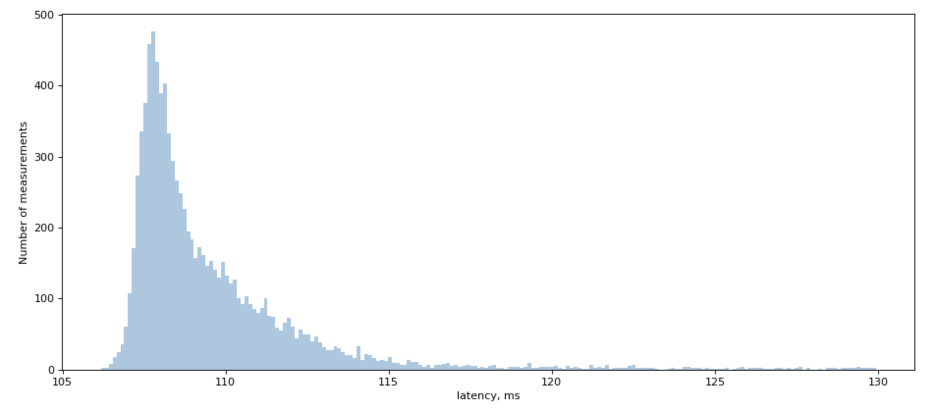
We often simplify things, saying that it’s a “lognormal” distribution, but if you try to fit lognoram distribution, you will find that real-world distribution has a very unplesant tail that doesn’t really want to be fitted.
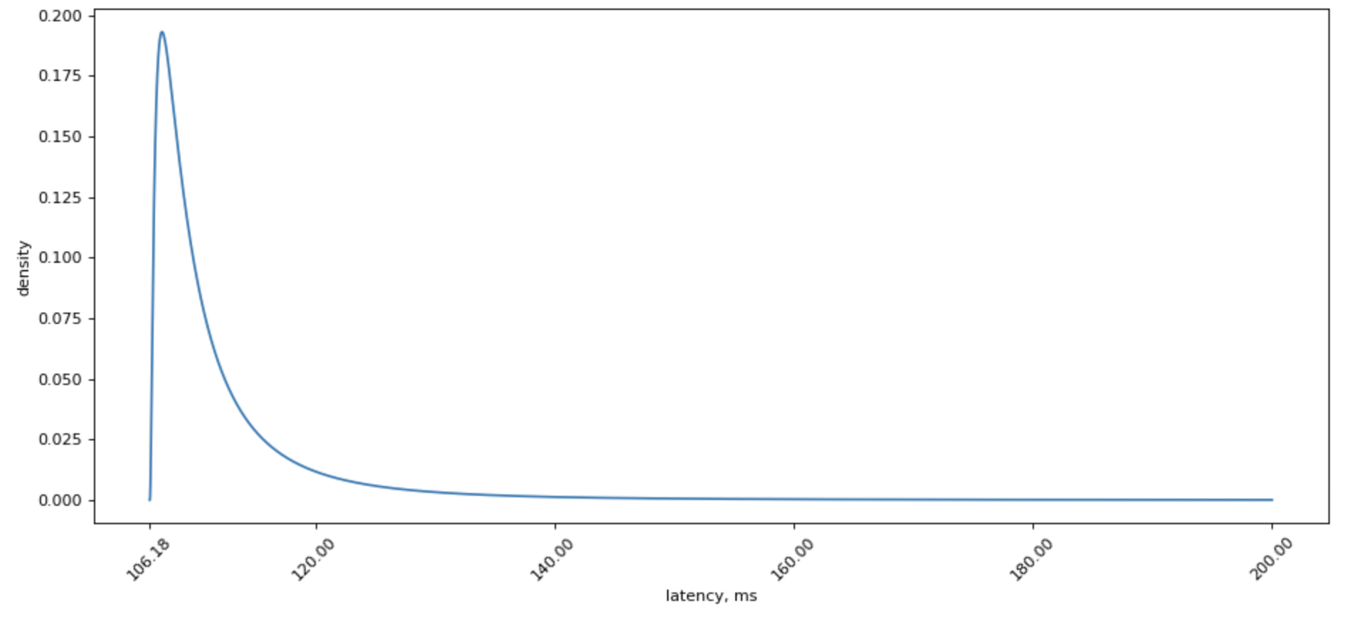
However, lognormal distribution is sure much prettier to look at:
Since we started speaking of tails, how do we measure one?
Easy! We can sort all our measurements, count 50% lowest latencies, and ask what is the highest latency for this group? We would also want this number of 50, 95, and 99 percentile, and sometimes 99.9. For shortness, we call it p50, p95, p99.
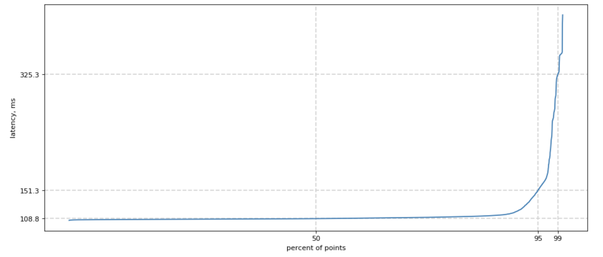
Poorly fitted, but much prettier chart for lognormal distribution looks like this:
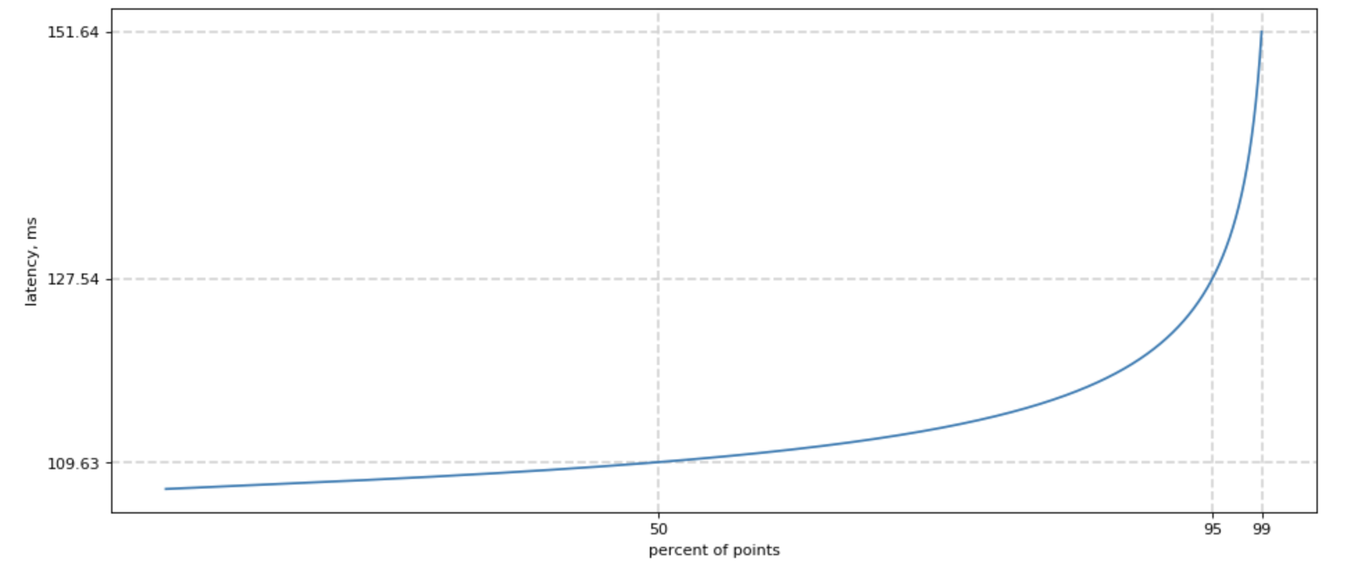
Overall p99 latency
When you show p99 over time for different backends it would most likely look something like this, if the servers have different loads:
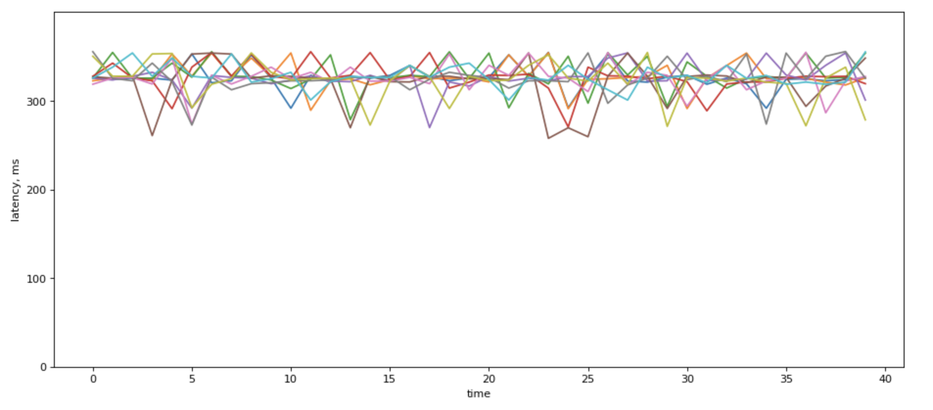
When there are a lot of lines in there, fight the urge to average over p99. It sure looks prettie:
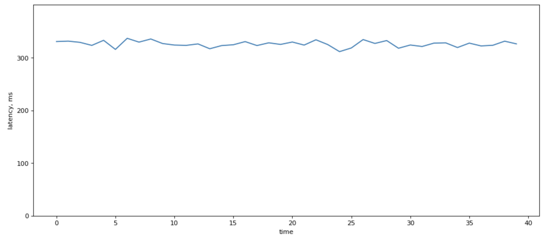
Howeer, it destroys information about load balancing among your servers.
One of the “right ways” to calculate system’s p99 latency is by using a sample of latencies across the system. But this can be burdensome.
May be the way is not to calculate it at all.
A good reason not to use average is to think about a couple of situations where averaging will give a very wrong results:
High p99 in part of the system
| Node | Latency | RPS |
|---|---|---|
| Node 1 | 100 ms | 1000 |
| Node 2 | 200 ms | 1000 |
If you sort their latencies, most likely, second node’s latencies would be so far to right compared to the first one, and the overall latency would be dominated by the second node. So the “true” p99 would be 200ms, but the average is just 150ms. Not great.
Unbalanced load
A second case, if you have unbalanced load profile, where one (some) of your nodes handle a higher load. That easily can happen in heterogeneous system with baremetal servers.
Consider two nodes from our distribution
| Node | Latency | RPS |
|---|---|---|
| Node 1 | 151 ms | 1000 |
| Node 2 | 78 ms | 10000 |
The average of that is (151+78)/2 = 114.5. But in reality, that can be just 80 ms, because Node 1 with high RPS would “dominate” the distriubiton.
Latency: from linear growth to exponential decay with number of backends
We’ve already discussed how do we measure latency and that we use p95, p99, and sometimes p999.
Let’s look at what happens when we have multiple backends. For simplicity, I’m going to use the same latency profile for all backends.
And you can think of these backends as redises.
Sequential access is not great.
Imagine that when request comes we handle it like this:
- Some logic
- Access microservice
- Some extra logic … N. response
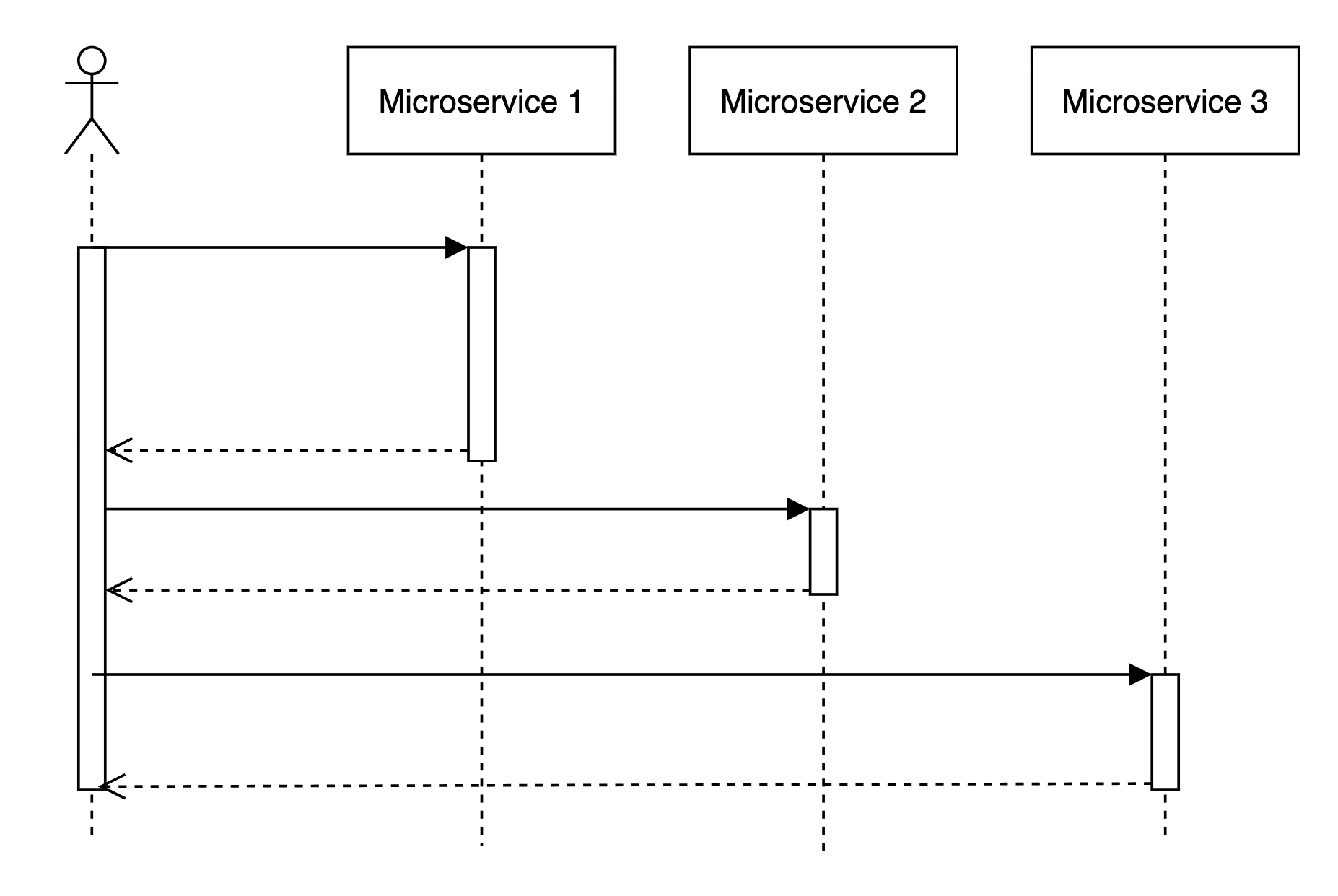
In this case, tail latencies will stack up in an expected linear manner.
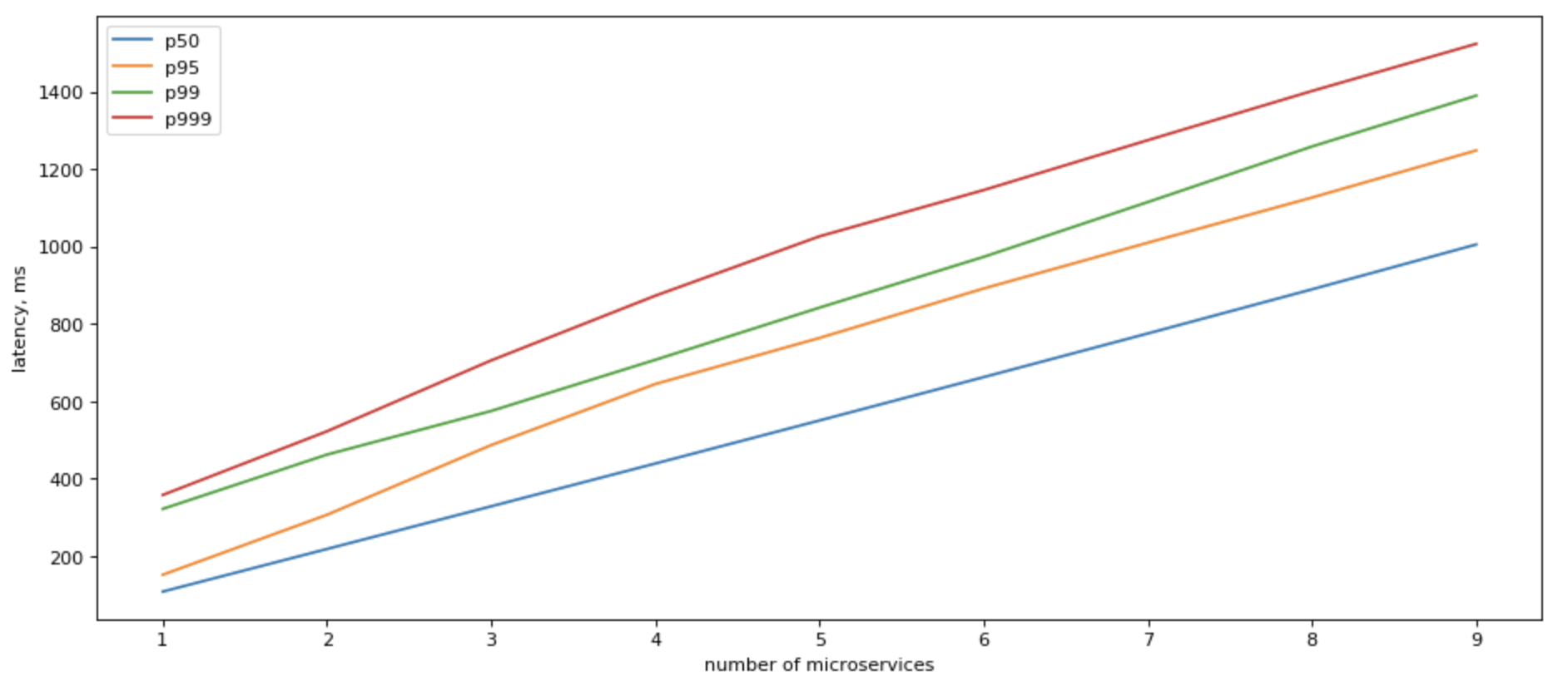
Can we do anything about it?
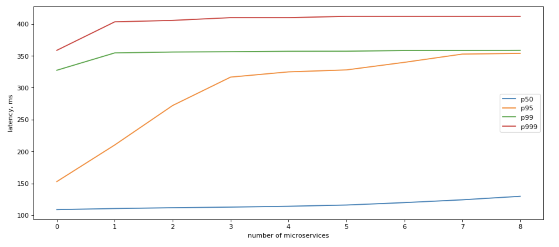
Yes, we can! If we can refactor our app to make parallel calls to all downstream microservices in parallel, our IO latency would be capped by the slowest response of a single service!
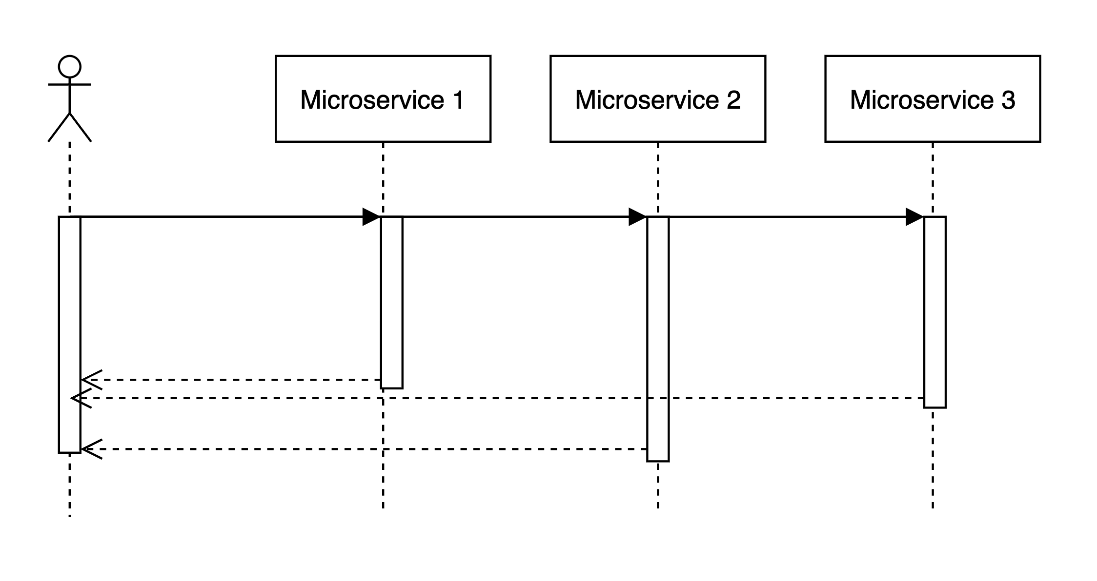
In that case, tail latency would grow roughly logarithmically with the number of backends:
If we look at what sequential IO gives us, the picture becomes clearer:
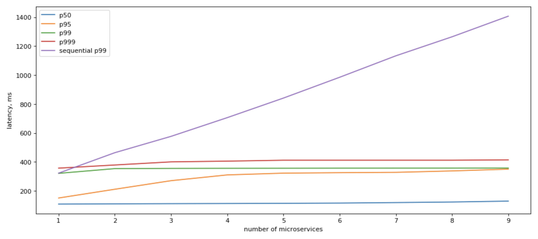
It still slower than having just 1 microservice to access, but it’s a very significant positive change.
Can we do something more about it?
Parallel microservices access
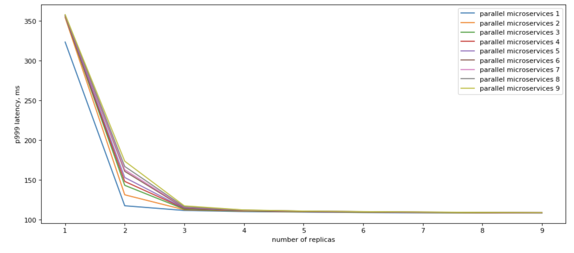
Yes, we can! If we can use multiple replicas, we can do parallel calls to all of them, and when we recieve the fastest answer, cancel all other in-flight requests, we would have a vey nice p99
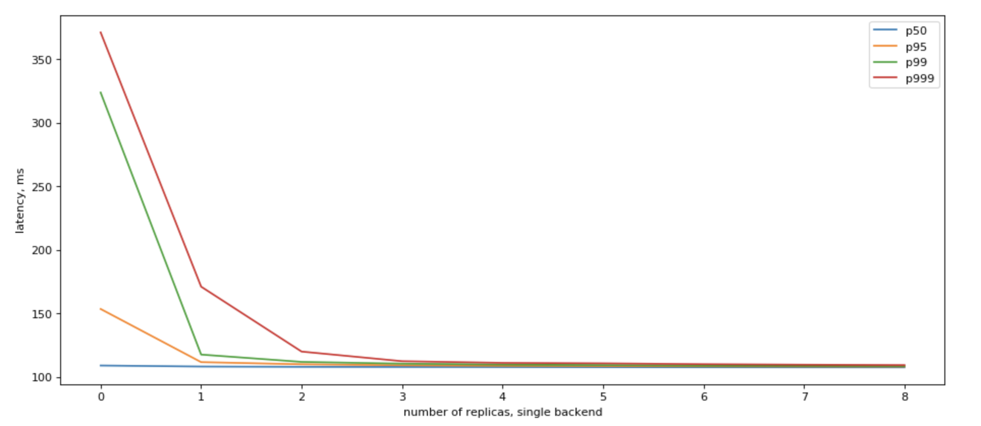
Please also note, that we get the most results by having just a few (3) read replicas.
Improving sequential microservices access
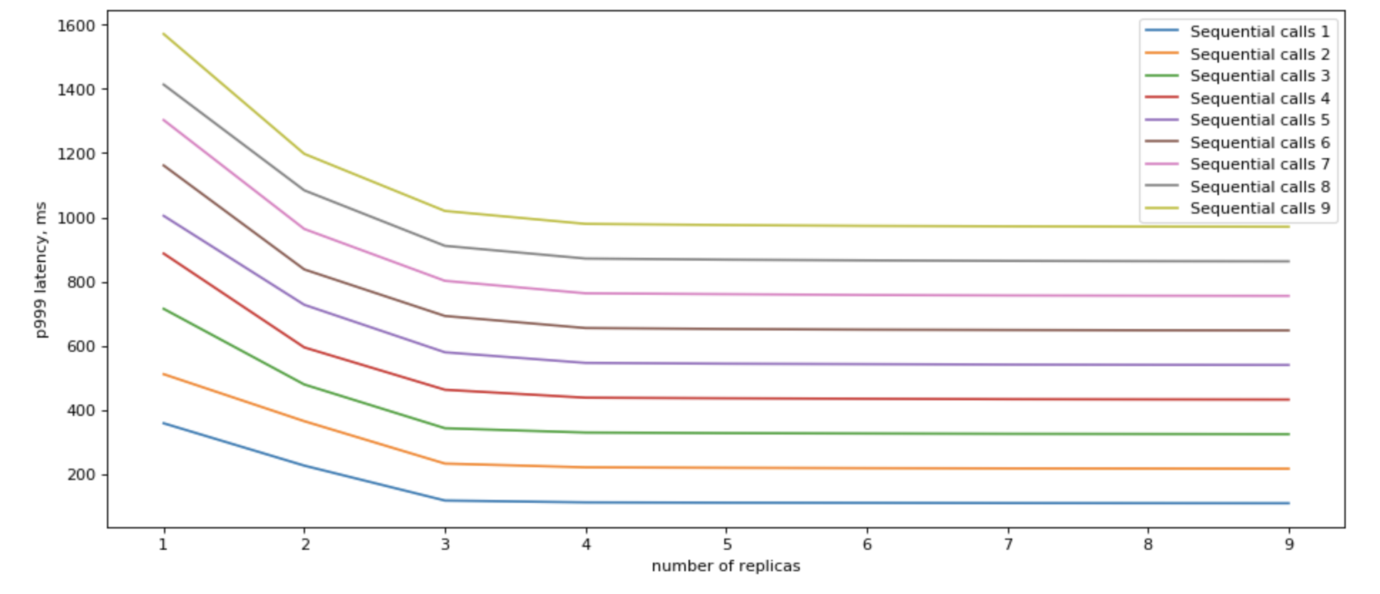
So for cases when we can’t change the sequetial matter of our code, we can add read replicas, and expect some imporovement, if we send requests to all read replicas in parallel, and as soon as we get first one (i.e. the fastest one), we go on.
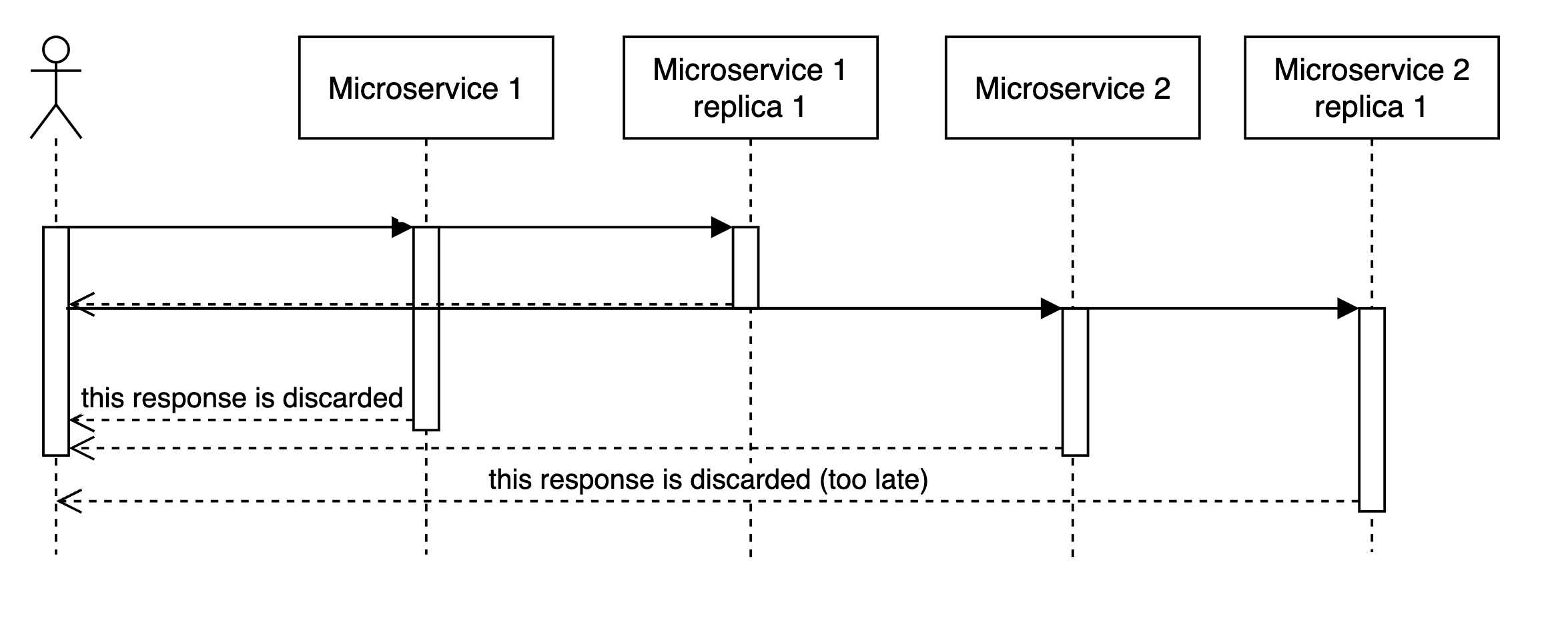
In general, looks like for practical purposes and a single backend, it does quite well at 2 read replicas.
But it’s not great.
Improving parallel microservices access
If you call multiple read replicas in parallel, you would get a remarkable improvement in terms of latency.
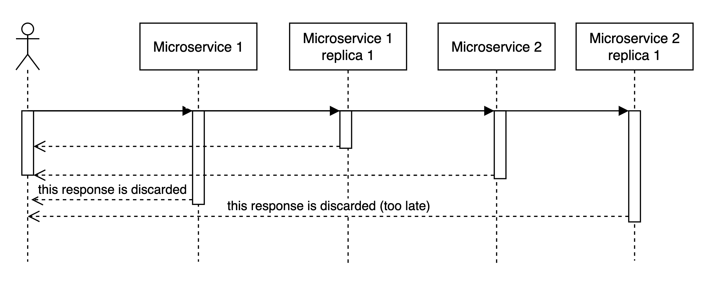
There are a few points to consider:
- We are already fast with parallel calls. Do we need to be faster? Is it worth it?
- We likely have replicas for fault tolerance. Can we use them as read-only replicas?
- Network overhead. If you are close to network stack saturation on your nodes, does it make sense to double or triple the load?
